gsw
Dan Kelley (https://orcid.org/0000-0001-7808-5911) and Clark Richards (https://orcid.org/0000-0002-7833-206X)
2024-08-19
Source:vignettes/gsw.Rmd
gsw.RmdAbstract. The gsw package provides an R
implementation of the Gibbs SeaWater toolbox for the calculation of
seawater properties, based on the GSW-C framework1. This vignette
outlines how to use gsw alone or as part of the
oce package (Kelley, Richards, and
Layton 2021).
Introduction
In recent years, thermodynamic considerations have led to improved
formulae for the calculation of seawater properties (IOC, SCOR, and IAPSO 2010; Millero 2010; Pawlowicz et
al. 2012), an important component of which is the Gibbs-SeaWater
(GSW) toolbox (McDougall and Barker 2020).
The gsw package is an R version of GSW, which may be used
independently or within the more general oce package (Kelley, Richards, and Layton 2021).
This vignette sketches how to use gsw. Readers are
assumed to be familiar with oceanographic processing, and at least
somewhat familiar with GSW. A good resource for learning more about GSW
is http://www.teos-10.org, which
provides technical manuals for the Matlab version of GSW http://www.teos-10.org/pubs/gsw/html/gsw_contents.html,
along with white papers and links to the growing peer-reviewed
literature on the topic.
The gsw framework uses function wrappers that connect R
with the C version of the Gibbs Seawater library. This yields high
processing speed. By minimizing transliteration errors, it also
increases reliability. In a further effort to increase reliability,
GSW-R makes tests against the check values provided on the webpages that
document GSW-Matlab.
By design, the documentation of gsw functions is spare,
amounting mainly to an explanation of function arguments and return
values, with most other details being provided through hyperlinks to the
GSW reference documentation. The idea is to avoid duplication and to
encourage users to consult the technical materials linked to the GSW
functions mimicked in gsw. The GSW system is somewhat
complex, and analysts owe it to themselves to learn how it works, and
also to develop an appreciation for its scientific context by consulting
various documents at http://www.teos-10.org, including
expansive white papers and pointers to the growing peer-reviewed
literature (Wright et al. 2011; McDougall and
Barker 2020; Graham and McDougall 2012).
Using gsw independent of oce
Suppose a water sample taken at pressure (For practical reasons,
gsw goes beyond SI to incorporate oceanographic units, such
as decibars for pressure.) 100 dbar, longitude 188E and latitude 4N,
reveals Practical Salinity 35 and in-situ temperature
10C
(ITS-90). Then the Absolute Salinity may be calculated as follows.
library(gsw)
SA <- gsw_SA_from_SP(SP=35, p=100, longitude=188, latitude=4)
This yields SA=35.1655491 [g/kg], which can then be used
to calculate Conservative Temperature as follows.
CT <- gsw_CT_from_t(SA=SA, t=10, p=100)The above yields CT=9.9782488
[C].
Readers familiar with GSW will recognize the function and argument
names, and are likely to find the other functions needed for their work
among the roughly sixty functions that gsw provides.
Using gsw within oce
Many oce plotting functions have an argument named
eos that can be set to the string "unesco" to
get the older seawater formulation, or to "gsw" to get the
newer one. For example, the section dataset provided by
oce holds a sequence of CTD casts in the North Atlantic.
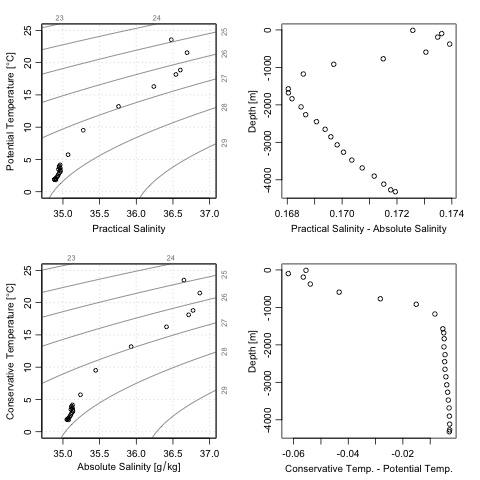
Individual casts may be selected by index, so a TS diagram of the
station at index 100 (south of Cape Cod in 4000 m of water) can be
plotted as follows.
library(oce)
data(section)
ctd <- section[["station", 100]]
Slim <- c(34.8, 37.0)
Tlim <- c(0, 25)
par(mfcol=c(2,2))
plotTS(ctd, Slim=Slim, Tlim=Tlim, eos="unesco")
plotTS(ctd, Slim=Slim, Tlim=Tlim, eos="gsw")
plot(ctd[["SA"]] - ctd[["salinity"]], ctd[["z"]],
     xlab="Practical Salinity - Absolute Salinity", ylab="Depth [m]")
plot(ctd[["CT"]] - ctd[["theta"]], ctd[["z"]],
     xlab="Conservative Temp. - Potential Temp.", ylab="Depth [m]")
Most hydrography-related functions of oce provide this
eos argument for selecting the seawater formulation. This
includes functions for plotting and for calculating. In addition, most
of the objects within oce have accessors that can return
temperature and salinity in either the UNESCO or GSW
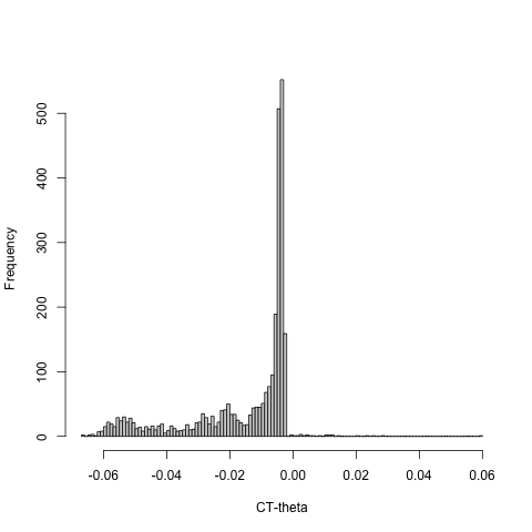
scheme. For example, the ratio of Conservative Temperature to
UNESCO-formulated potential temperature
for all the CTD profiles in section is constructed with
f <- section[["CT"]] - section[["theta"]]
hist(f, main="", breaks=100, xlab="CT-theta")
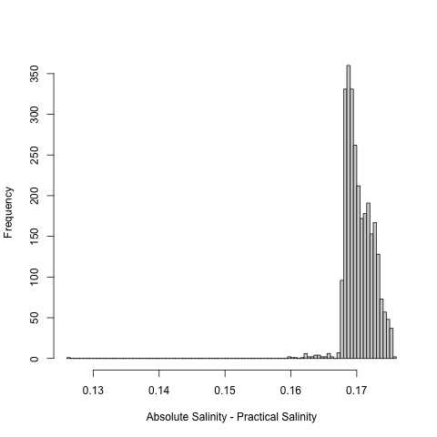
A salinity comparison is constructed with
f <- section[["SA"]] - section[["salinity"]]
hist(f, main="", breaks=100, xlab="Absolute Salinity - Practical Salinity")
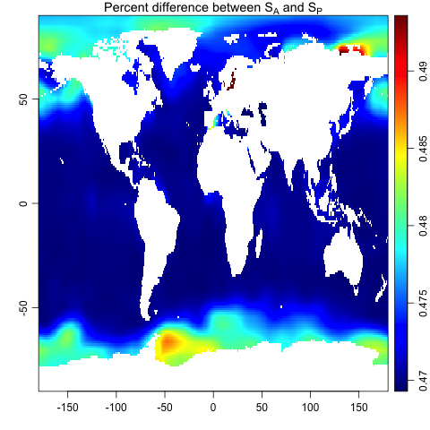
An examination of worldwide spatial patterns is also informative, with the following producing such a graph.
library(oce)
data("levitus", package="ocedata")
SSS <- levitus$SSS
dim <- dim(SSS)
ll <- expand.grid(lon=levitus$longitude, lat=levitus$latitude)
SA <- gsw_SA_from_SP(levitus$SSS, 0, ll$lon, ll$lat)
per <- 100 * (1 - levitus$SSS / SA)
imagep(levitus$longitude, levitus$latitude, per, col=oceColorsJet,
       zlim=quantile(per, c(0.001, 0.999), na.rm=TRUE))
title(expression("Percent difference between " * S[A] * " and " * S[P]))
Note the use of quantile-specified scales for the images, the colour mappings of which would otherwise be controlled by isolated low-saline waters, yielding little to see in the wider expanses of the world ocean; for a broader context, see e.g. McDougall and Barker (2020).
